Initial Conditions and Parameters
The code begins by setting up the computational grid and initial conditions. The spatial domain is discretized into grid points with dx and dy representing the spacing between these points in the horizontal and vertical directions, respectively. Several matrices such as XINEW, XIOLD, P, U, and V are initialized to store the stream function, pressure, and velocity components at each grid point. The physical dimensions of the domain are defined by L (length) and H (height), and the angle LPHA potentially represents the orientation of the valve-like obstruction within the flow domain. The grid resolution is determined by IL (horizontal grid points) and JL (vertical grid points). The variables Start_x, Start_y, End_x, and End_y likely represent the coordinates defining the location and extent of the obstruction within the flow domain.
%Initial Conditions
dx = 0.005;
dy = 0.005;
XINEW = zeros(41, 201);
XIOLD = zeros(41, 201);
P = zeros(41, 201);
U = zeros(41, 201);
V =zeros(41, 201);
L= 1; %meters
H= 0.2; %meters
LPHA = pi/4;
IL = 201; %Horizonil grid points
JL = 41; %Verticl grid points
Start_x = round((L/2 - (H/2 *sin(LPHA)) )/dy);
Start_y = round((H/2 - (H/2 *cos(LPHA))  )/dx);
End_x = round((L/2 + (H/2 *sin(LPHA))    )/dy);
End_y = round((H/2 + (H/2 *cos(LPHA))   )/dx);
Simulation Parameters
The code sets several key simulation parameters such as the maximum number of iterations (NMAX), the freestream density (ROINF), pressure (PINF), and velocity (UINF). The relaxation factor (OMEGA) and the acceptable error (ERR) are specified to control the iterative solution process.
NMAX = 100000;% max number of iterations
ROINF= 1; %kg.m^3
PINF = 100000; %Pa
UINF = 50; %m/s
OMEGA =  1.5;
ERR = 10^-4;%Acceptable error
n = 0;
Initial Flow Field Setup
The code initializes the flow field by setting a linear distribution of the stream function (XI) across the vertical dimension of the domain, assuming a simple flow profile that ignores the presence of the obstruction. This initial setup serves as a starting point for the iterative solution process.
for J = 1:JL
    XI = UINF * H *((J-1)/(JL-1)); %Initial streamfunctions through tube, ignores presence of vLve
    for I = 1:IL
        XIOLD(J,I) = XI;
        XINEW(J,I) = XI;
    end
end
XI = 0.5 * H * UINF; %Streamfunction Long vLve
Iterative Solution Process
The core of the simulation is an iterative process that updates the flow field to account for the presence of the obstruction. The code uses a relaxation technique, indicated by the use of the OMEGA parameter, to progressively update the stream function values (XINEW) across the domain. This process involves updating the stream function in different sections of the flow domain, taking into account the obstruction's geometry. The convergence of the solution is monitored using a normalized sum of squared differences between successive iterations of the stream function values (SNORM). The iterative process continues until this error metric falls below the predefined acceptable error (ERR) or until the maximum number of iterations (NMAX) is reached.
hile (n < NMAX) %iterate through interior points
    for IR = Start_x : End_x %Range horizantly for vive
        JR = round(End_y -(IR - Start_x)); %Appropriate j vLue for i vLue of vLve
        XIOLD(JR,IR) = XI;
        XINEW(JR,IR) =  XI;
    end

    for J = 2:JL - 1 %First section before vLve
        for I = 2:(Start_x-1)
            XINEW(J,I) = 0.25*(XINEW(J-1,I)+XINEW(J,I-1)+XIOLD(J+1,I) +XIOLD(J,I+1));
            XINEW(J,I) = OMEGA*XINEW(J,I)+(1-OMEGA)*XIOLD(J,I);
        end
    end
    Jrange = End_y;
    for I = Start_x:End_x-1 %Second Section above vLve
        for J = 2: Jrange-1
            XINEW(J,I) = 0.25*(XINEW(J-1,I) + XINEW(J,I-1) +XIOLD(J+1,I) + XIOLD(J,I+1));
        end
        Jrange = Jrange - 1;
    end
    Jrange = End_y-1;
    for I = Start_x + 1:End_x-1 %Third Section above vLve
        for J = Jrange + 1:JL-1
            XINEW(J,I) = 0.25*(XINEW(J-1,I) + XINEW(J,I-1) + XIOLD(J+1,I) + XIOLD(J,I+1));
        end
        Jrange = Jrange - 1;
    end
    for J = 2:JL-1 %Fourth Section above vLve
        for I = End_x+1:IL -1
            XINEW(J,I) = 0.25*(XINEW(J-1,I) + XINEW(J,I-1) + XIOLD(J+1,I) + XIOLD(J,I+1));
            XINEW(J,I) = OMEGA*XINEW(J,I) +(1-OMEGA)*XIOLD(J,I);
        end
    end
    SNORM = 0;
    for J = 2:JL-1
        for I = 2:IL -1
            SNORM = SNORM + ((XINEW(J,I) - XIOLD(J,I))/XINEW(J,I))^2;
        end
    end
    SNORM = SNORM/((IL -1)*(JL-1));
    if SNORM < ERR
        n = NMAX;
    else
        n = n+1;
    end
    for J = 2:(JL-1)
        for I = 2:(IL-1)
            XIOLD(J,I) = XINEW(J,I);
        end
    end
end
Post-Processing
After the iterative process completes, the code calculates the velocity components (U, V) and pressure distribution (P) across the domain based on the final stream function values. These calculations involve spatial derivatives of the stream function, consistent with fluid dynamics principles.
XINEW2 = zeros(size(XINEW));
for J  = 1:1:JL
    XINEW2(J,:) = XINEW((JL+1)-J,:);
end

for J = 2:JL-1
    for I = 2:IL - 1
        U(J,I) = ((XINEW(J+1,I) - XINEW(J-1,I))/(2*dy));
        V(J,I) = -((XINEW(J,I+1) - XINEW(J,I-1))/(2*dx));
    end
end

U(1,1) = UINF;
V(1,1) = 0;
V(JL,IL) = UINF;
V(JL,IL) = 0;

    for IR = Start_x:End_x
        JR = round(End_y - (IR-Start_x));
        U(JR,IR) = 0;
        V(JR,IR) = 0;
    end
for J = 1:JL
    for I = 1:IL
        P(J,I) = PINF +(0.5*ROINF*(UINF^2)) - (.5*ROINF*((U(J,I)^2) +(V(J,I)^2)));
    end
end

XI = 0.5 * H * UINF; %Streamfunction Long vLve
Visualization
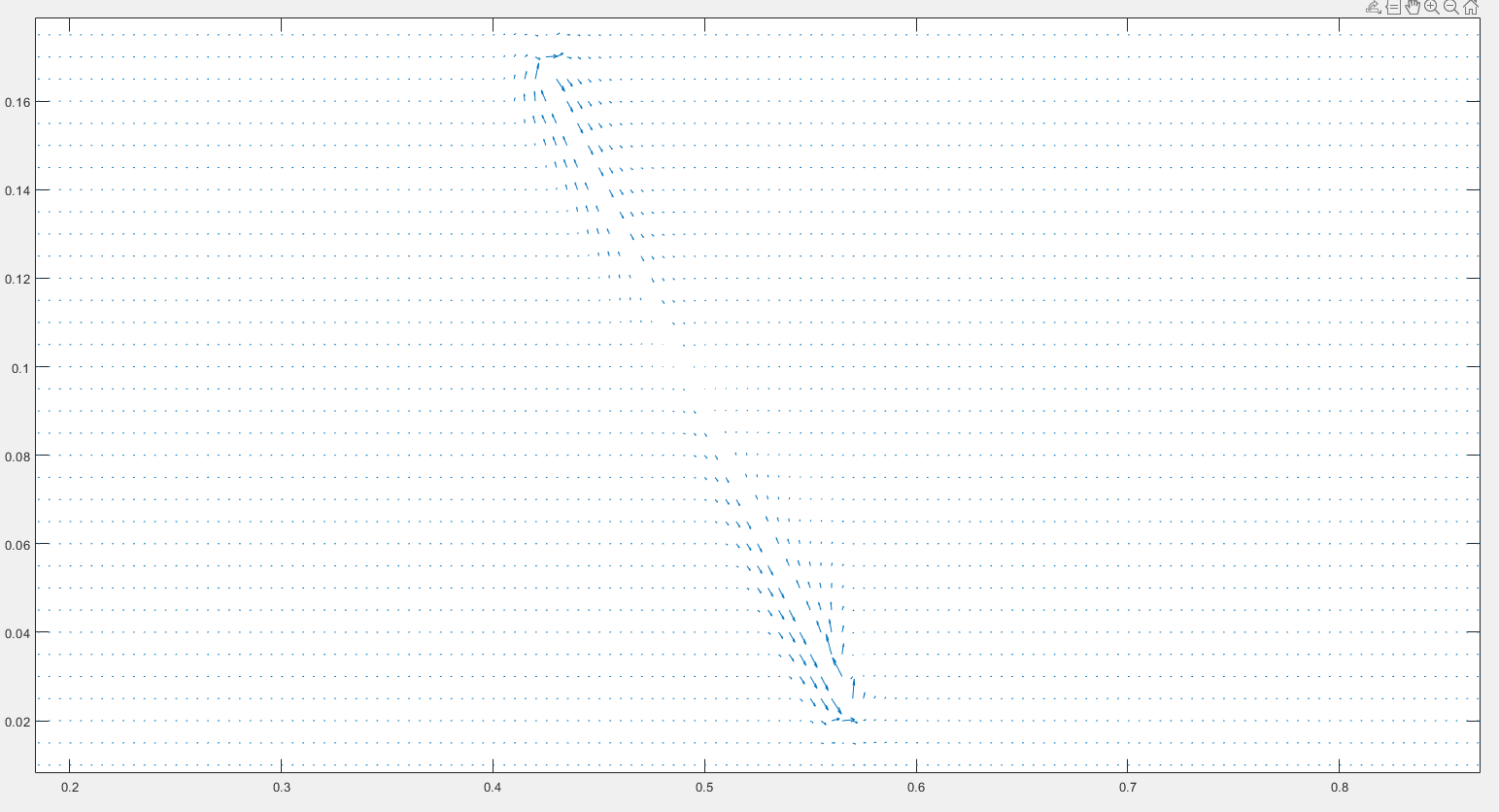
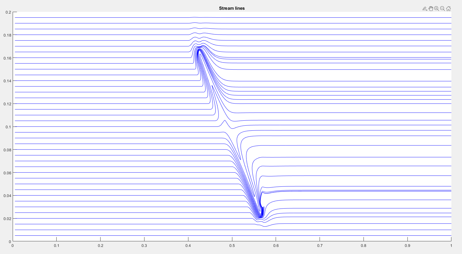
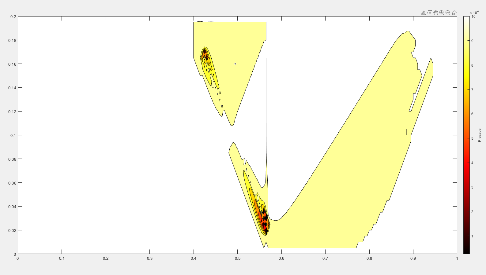
The code concludes with the generation of visualizations to represent the simulation results. This includes quiver plots to visualize the velocity field, streamline plots to visualize the flow paths, and contour plots to visualize the pressure distribution. These visualizations provide insights into the fluid flow behavior, particularly around the obstruction, and are crucial for analyzing the simulation results.
[x,y] = meshgrid(0:dx:L,0:dy:H);

figure(1)
quiver(x,y,U,V);
starty = 0:dy:H;
startx = dx*ones(size(starty));
figure(2)
streamline(x,y,U,V,startx,starty);

figure(3)
contourf(x,y,P)
colormap(hot)


Conclusion
This CFD code offers a detailed simulation of fluid flow through a domain with a specific geometric feature that influences the flow pattern. Through iterative updates and post-processing, the code provides valuable insights into the flow characteristics, which are essential for understanding the fluid dynamics within the specified domain.